Difference Between Fisher Exact Test and Chi Square Updated

Difference Between Fisher Exact Test and Chi Square

This article aims to introduce the statistical methodology backside chi-square and Fisher'due south verbal tests, which are commonly used in medical research to assess associations between categorical variables. This discussion volition use information from a study by Mrozek ¹ in patients with astute respiratory distress syndrome (ARDS). This was a multicenter, prospective, observational study: multicenter considering it included data from 10 intensive intendance units, prospective because the study collected the information moving forward in time, and observational because the study investigators did non have control over the group assignments but rather used the naturally occurring groups. The study objective was to characterize focal and nonfocal patterns of lung computed tomography (CT)-based imaging with plasma markers of lung injury.

The main grouping variable was type of ARDS (focal vs nonfocal) as determined by CT scans and other lung imaging tools. In this study, there were 32 (27%) patients with focal ARDS and 87 (73%) patients with nonfocal ARDS. What will be of import, however, is classifying the blazon of variables because this determines the blazon of analyses performed. Type of ARDS is a categorical variable with 2 levels.

The primary study endpoint was plasma levels of the soluble form of the receptor for advanced glycation end product. In that location were also a number of secondary study endpoints that can be grouped every bit either patient outcomes or biomarkers. Patient outcomes included the elapsing of mechanical ventilation and both 28- and 90-day mortality. Levels of other biomarkers included surfactant protein D, soluble intercellular adhesion molecule-ane, and plasminogen activator inhibitor-ane.

This article focused on the secondary result of ninety-day mortality beginning at illness onset. Again, we are interested in classifying this variable, which is categorical with 2 levels (yes vs no). So the scenario is that we want to assess the relationship between the type of ARDS (focal vs nonfocal) and 90-24-hour interval mortality (yes vs no). In its most basic form, this scenario is an investigation into the clan amongst 2 categorical variables.

When there are ii categorical variables, the information tin be arranged in what is called a contingency tabular array (Figure ane). Because both variables are binary (ii levels), information technology is chosen a two × 2 table. Withal, a contingency table tin can be generated for 2 categorical variables with any number of levels—in that case, it is chosen an r × c table, where r is the number of levels for the row variable and c is the number of levels for the column variable. The actual raw counts or frequencies are recorded inside the table cells. The cell counts are often referred to as observed counts and thus the notation (O_ij) is used. The subscript i identifies the specific level of the row variable, and in this example information technology can equal one or two since the row variable is binary. Similarly, the subscript j identifies the specific level of the cavalcade variable and in this example it tin can equal ane or 2 since the column variable is binary. Therefore, O₁₁ represents the number of patients who take the row variable = level 1 and the column variable = level one.

In addition to the row and column variable cells, there are also the margin totals. These totals are either the row margin total (summing across the row) or the cavalcade margin total (summing down the column). For instance, n₁₊ is the sum of the row where the row variable equal 1 (O₁₁ + O₁₂ = n₁₊). Finally, at the very bottom right corner is the grand full, which equals the sample size.

The goal is to test whether or non these 2 categorical variables are associated with each other. The nada hypothesis (H_o) is that there is no association between these 2 categorical variables and the culling hypotheses (H_a) is that there is an association between these 2 categorical variables.

The adjacent step is to translate the generic form of the hypotheses into hypotheses that are specific to the research question. In this case, the null hypothesis is that mortality is not associated with lung morphology and the alternative hypothesis is that mortality is associated with lung morphology.

The contingency table cells tin be populated with the numbers constitute in the article. It has our outcome of focus—mortality at twenty-four hours 90—both the count and the percent. The results are broken downwards past type of ARDS (focal vs nonfocal) as follows:

• Focal ARDS = half dozen patients (21.4%)

• Nonfocal ARDS = 35 patients (45.five%).

From these numbers, we tin can build the contingency table that corresponds to the clan among lung morphology (type of ARDS) and 90-day bloodshed (Figure ii).

Offset, the row variable is lung morphology, and it has two levels (focal vs nonfocal). Next, the column variable is xc-mean solar day mortality and it has 2 levels (yes vs no). Finally, the table must exist populated, merely exist careful not to assume that there are no missing data. Begin with the cell counts: at that place were half-dozen focal ARDS patients and 35 nonfocal ARDS patients who died within xc days. These two numbers populate the get-go column and effect in a column total of 41. Side by side, use the reported percentages to summate the row totals. Six is 21.4% of 28, so the first row full is 28. Thirty-five is 45.5% of 77, and so the second row total is 77. If at that place are 28 patients with focal ARDS and 77 with nonfocal ARDS, and then the 1000 total is 28 + 77 = 105. The remaining values can be obtained by subtraction. If there are 105 total patients and 41 die within 90 days, then 105 − 41 = 64 patients who do not die within 90 days and this is the 2nd column full. Similarly, if at that place are 28 focal ARDS patients and 6 die inside 90 days, then 28 − half dozen = 22 patients who do not die inside 90 days. Lastly, if there are 77 nonfocal ARDS patients and 35 die within 90 days, then 77 − 35 = 42 patients who do not dice within 90 days. Now the contingency tabular array is complete.

Once the contingency table is built, the question becomes, "Is lung morphology associated with ninety-24-hour interval mortality?" To answer that question, we need to know how many patients one would wait in each table jail cell if the null hypothesis of no association is true. When conducting a hypothesis examination, one e'er assumes that the cipher hypothesis is true and then gathers information to meet how well the data aligns with that assumption.

And so one must summate how many patients to expect in each of these cells if lung morphology is not associated with 90-day mortality. One way to accost this question is to ask these two questions:

1. Overall, what proportion of patients dice by day 90? Looking at the constructed contingency table, that answer would be 39%. This was calculated by taking the total number of patients who died by twenty-four hours 90 and dividing it by the total number of patients, 41/105 = 39%. This gives the overall proportion, based on the data, who would die by day 90.

2. How many of the focal ARDS patients would be expected to die by day 90? Now it is non overall, only rather we are limiting the question to the focal ARDS grouping. To obtain the answer, multiply the overall proportion of patients who die by day 90 by how many focal ARDS patients are in the study. Substantially, take the respond from the previous question and multiply it by the full number of focal ARDS, which is 28. The result is (41/105) × 28 = 10.9. Thus, if in that location is no association among long morphology and xc-day mortality, one would expect 10.9 focal ARDS patients to die by twenty-four hour period 90.

Now 10.9 is a very specific answer for a specific contingency table, simply the answer could be written in general terms. Basically, 3 numbers were used in calculating the solution: the row margin, the column margin, and the thou total. The general formula is the following:

The notation Due east_ij is used to represent the expected count assuming the null hypothesis of no clan amongst the row and column variables is true. To summate the expected count, have the i ^thursday row total times the j ^thursday column total and divide by the grand total.

In the lung morphology and bloodshed case, what is the expected number of deaths within 90 days amongst the nonfocal ARDS patients? This is the second row and the first column (Eastward₂₁). Applying the formula, one multiplies the full for the 2d row by the full for the first cavalcade and then divides by the chiliad total, (77 × 41)/105 = xxx.one. This calculation is repeated for each of the 4 cells.

Because we at present know the observed prison cell count and the expected cell count (under the cipher hypothesis), nosotros can compare the observed and expected counts to run into how well the information aligns with the null hypothesis. This is what the chi-square test does, and the test statistic is calculated equally follows:

The sigma (Σ) means addition, so the adding is performed on each individual prison cell in the contingency tabular array and so the results are summed. A 2 × ii tabular array has 4 cells and thus 4 numbers will exist summed. For each cell, the formula compares the observed to the expected. Basically, it computes how like they are (that is the O minus E part). Because the differences will be positive for some cells and negative for others, the differences are squared to avoid cancellation when yous add them. Finally, each squared divergence is divided by the expected count to standardize the calculation.

Intuitively, if the observed counts (O_ij) are similar to the expected counts under the null hypothesis (E_ij), then these 2 numbers will be very close to each other. When taking the difference between them or subtracting them, the effect is a small number. When squaring a small number, one obtains a really small-scale number. And adding upwardly a agglomeration of really small numbers results in a small number. So the examination statistic is going to be small-scale. That means that the resulting P value is going to be large. What is a P value? Think of information technology as an index of compatibility. How compatible is the data with the cypher hypothesis? Here, you get a large alphabetize of compatibility. That means that the data aligns nicely with the nil hypothesis and one fails to turn down the nix.

Now, think about the culling scenario. If the observed counts (O_ij) are wildly unlike from the expected counts under the goose egg hypothesis (Eastward_ij), then these 2 numbers will be quite different. When taking the departure betwixt them or subtracting them, the result is a big number. When squaring a large number, one obtains a really big number, and calculation up a bunch of really big numbers results in a large number. So the test statistic is going to exist big. That means that the resulting P value is going to be small. And if you lot call up of a P value every bit an index of compatibility, the data and the null hypothesis are non very compatible. That means that the data does non align nicely with the zilch hypothesis and one rejects the cypher. This is the general thought of the chi-square test. It assesses how compatible the data is with the nothing hypothesis that the 2 chiselled variables are not associated.

To obtain the bodily P value, the distribution of the test statistic (under the nil hypothesis) is used to calculate the area under the curve for values equal to the exam statistic or more extreme. The described test statistic has an estimate chi-square distribution with (r − one)(c − 1) degree of freedom. Recall that r is the number of levels of the row variable and c is the number of levels of the column variable. Our example is a 2 × 2 table, so the examination statistic has an approximate chi-square distribution with (2 − 1)(2 − 1) = 1 degree of liberty.

At present that the chi-square test has been fully described, the assumptions for the test must exist discussed. It is important to know when you should or should not perform this test. The chi-square test assumes that observations are independent. This means that the consequence for one ascertainment is non associated with the outcome of any other observation. This principle can be violated when multiple measurements are taken over time or when multiple measurements are taken from one patient.

Another assumption is that the chi-square large sample approximation only described is appropriate. In other words, no more than than 20% of the expected counts (E_ij) are less than 5. For a 2 × ii table, how many cells do you lot have? Iv. And so if even one of those 4 happens to take an expected count less than five, this assumption is violated. For a 2 × 2 table, none of the expected counts can be less than five.

Returning to the lung morphology and bloodshed example, were the assumptions met? The data consist of 105 unique patients. Thus, we can assume that they are contained. The minimum expected count was 10.nine, which is not less than 5. Therefore, the assumptions for the chi-square examination are met. Adjacent, the examination statistic is calculated using the observed and expected counts. For each jail cell, subtract the expected count from the observed count, foursquare information technology, and divide by the expected count. Then, add the 4 resulting numbers to obtain the test statistic of 4.92.

Finally, compute the area under the chi-square distribution with one degree of freedom, χ² _(i), at the test statistic and values more farthermost. In this case, values more farthermost are values greater than the test statistic. Here, the area under the curve to the right of 4.92 is .027 (Effigy three). This is the P value, which indicates that the information and the zippo hypothesis accept very low compatibility. In this case, the area under the curve to the correct of 4.92 is .027 (Effigy 3). This is the P value, which indicates that the data and the cypher hypothesis have very low compatibility. Thus, the decision is to reject the nix hypothesis. The conclusion is that lung morphology is associated with 90-day mortality (P = .027). To describe that association, one looks at the contingency table and finds a reduction in 90-day mortality with focal patterns compared to nonfocal patterns (21.4% vs 45.five%, respectively). The P value reported in the article is .026. Our hand calculation was .027, which is slightly off due to rounding. In summary, the scenario is an investigation into the association among 2 chiselled variables, and, thus, a exam to consider is the chi-square exam, if assumptions are met.

In another case in the same report, the authors investigate whether whatsoever baseline characteristics are associated with lung morphology. For example, is neurology, specifically Parkinson illness (yes vs no), associated with lung morphology (focal vs nonfocal)? Once again, the scenario is an investigation into the association between 2 categorical variables, so a chi-square test should be considered.

To starting time, build a contingency tabular array arbitrarily placing lung morphology as the row variable and Parkinson disease every bit the column variable. Populate the contingency table based on the counts and percentages reported in the article (Figure 4). Next, bank check that the assumptions of the chi-foursquare test are met. Are the observations contained? Again, because these are unique patients, we consider this assumption met. Since this is a 2 × 2 table, are all of the expected counts greater than five? Calculations of the expected counts obtained the following: i.ane, 30.9, 2.9 and 84.1. Here, 2 of the 4 expected counts are less than five. Therefore, methods that use large sample approximation, like the chi-squared test, may non be an appropriate selection.

Instead of using methodology that is an approximation, consider an exact exam such as Fisher's exact examination. Once more, refer to the contingency table where Fisher's exact is going to calculate the exact probability (nether the cipher hypothesis) of the observed data or results more than farthermost. This is the technical definition of a P value. It is, yet, even so quantifying how compatible the information are with the aught hypothesis. The exact probability of a particular contingency table tin can be obtained using the hypergeometric distribution.

The symbols that resemble big parentheses are notations for a combinatorial. Because using combinatorials to calculate the probability is non user friendly, an equivalent version relies on factorials instead. Both techniques are presented above. Remember that the goal is to find the verbal probability of the observed data or something more extreme.

The hypotheses are however testing whether these 2 categorical variables are associated with each other. In this detail example, nosotros test if the proportion of patients with Parkinson disease is the same in the focal and nonfocal groups. Fisher's verbal test obtains its two-tailed P value past computing the probabilities associated with all possible tables that have the same row and column totals. Then, it identifies the alternative tables with a probability that is less than that of the observed tabular array. Finally, it adds the probability of the observed table with the sum of the probabilities of each alternative table identified above, which results in the P value.

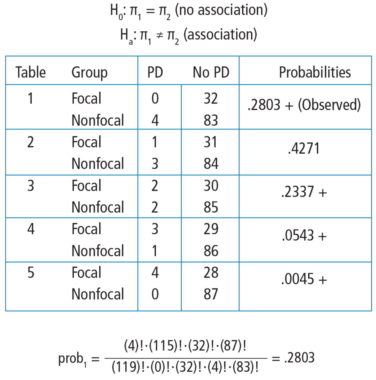
To explore each of those steps in detail, one must start enumerate how many tables can exist built that all have the aforementioned row and column totals as the observed table. Figure 5 shows the 5 possible tables. Pick any i of the 5 2 × two tables; the margins are fixed. Each table has the same row totals, 32 focal and 87 non-focal, and each table has the aforementioned column totals: 4 Parkinson and 115 non-Parkinson. Then, for each table, summate the probability of that tabular array. Figure five shows this calculation for the first two × 2 table, which happens to exist the observed table. The probability of the table observed in the written report is .2803. Such a adding is performed on each of the other tables.

P value is obtained by summing the probabilities of the observed tabular array and those more than extreme.

" data-icon-position="" data-hide-link-title="0">

• Download figure
• Open in new tab
• Download powerpoint

FIGURE 5

Mitt calculations of the Fisher's exact test. Note that all tables have the same row and column totals. The probabilities of each table are calculated according to the hypergeometric distribution. Tables deemed "more extreme" (ie, with probabilities < the observed tabular array) are indicated with a +. The P value is obtained past summing the probabilities of the observed tabular array and those more extreme.

Next, one must identify the tables that accept a probability smaller than the observed tabular array. Here, we are looking for probabilities less than .2803. These are the tables deemed more extreme. Tables 3, 4, and 5 take probabilities less than .2803.

The final step is to sum the probability of the observed table and the more extreme tables (ie, those with probabilities < the observed table) (.2803 + .2337 + .0543 + .0045 = .5728). Thus, the resulting rounded P value is .57, which indicates a high level of compatibility between the data and the cipher hypothesis of no association. The decision is to neglect to pass up the aught hypothesis and the conclusion is that the evidence does not back up an association among lung morphology and Parkinson illness. In other words, there is insufficient evidence to claim that the proportion of Parkinson disease differs between the focal and nonfocal ARDS patients (0% vs five%, P = .57). This matches the P value reported by Mrozek for this association.

The kickoff objective of this article was to identify scenarios in which a chi-foursquare or Fisher's exact test should be considered. The general setting discussed was an investigation of the clan between two categorical variables. Use of each examination specifically depends on whether the assumptions have been met. Both of the examples used in our word happened to be binary, only that is not a brake. Categorical variables tin have more than two levels. All of the methods demonstrated for ii × 2 tables tin exist generalized to r × c tables.

The second objective of this article was to recognize when test assumptions have been violated. For simplicity, most researchers adhere to the following: if ≤ twenty% of expected jail cell counts are less than v, then use the chi-square exam; if > 20% of expected cell counts are less than five, and so apply Fisher's exact test. Both methods assume that the observations are independent. Could one use the exact test when the chi-square assumptions are met? Yes, but it is more computationally expensive every bit information technology uses all possible stock-still margin tables and their probabilities. If the chi-foursquare assumptions are met, and then the sample size is typically larger and these calculations become numerous. Too, information technology does non have to exist that big of a sample for the chi-square to be a good approximation and do information technology very chop-chop.

The final objective of this article was to exam claims fabricated regarding the association of 2 independent categorical variables. We included examples from the medical literature showing step-by-footstep calculations of both the large sample approximation (chi-square) and exact (Fisher's) methodologies providing insight into how these tests are conducted also as when they are appropriate.

Footnotes

• This article is based on Dr. Nowacki's presentation at the "Biostatistics and Epidemiology" lecture series created by Aanchal Kapoor, Doctor, Critical Intendance Medicine, Cleveland Clinic. Dr. Nowacki presented her lecture on January x, 2017, at Cleveland Clinic.

• Dr. Nowacki reported no financial interests or relationships that pose a potential conflict of interest with this commodity.

• Copyright © 2017 The Cleveland Clinic Foundation. All Rights Reserved.